
Table of Contents
Our article delves into the world of DELL stock analysis. We’ll examine its past performance, current market conditions, and future potential. Whether you’re an experienced investor or just starting, this exploration promises valuable insights into DELL’s financial landscape. Let’s begin our journey.
Lets Start
import numpy as np # linear algebra
import pandas as pd # data processing, CSV file I/O (e.g. pd.read_csv)

# Input data files are available in the read-only "../input/" directory
# For example, running this (by clicking run or pressing Shift+Enter) will list all files under the input directory

import os
for dirname, _, filenames in os.walk('/kaggle/input'):
    for filename in filenames:
        print(os.path.join(dirname, filename))
Stock Analysis of DELL Stock
1. Import Libraries
import pandas as pd
import numpy as np

import matplotlib.pyplot as plt
import seaborn as sns
sns.set_style('whitegrid')
plt.style.use("fivethirtyeight")
%matplotlib inline

# For reading stock data from yahoo
from pandas_datareader.data import DataReader

# For time stamps
from datetime import datetime
from math import sqrt
from math import sqrt
from sklearn.metrics import mean_squared_error
from sklearn.preprocessing import MinMaxScaler

#ignore the warnings
import warnings
warnings.filterwarnings('ignore')

DE_Data = pd.read_csv('../input/dell-stock-data-latest-and-updated/DELL_stock_history.csv',sep='\t')

DE_Data.columns
Out[4]
Index([‘Date’, ‘Open’, ‘High’, ‘Low’, ‘Close’, ‘Volume’, ‘Dividends’, ‘Stock Splits’], dtype=’object’)
DE_Data.head()
Out[5]:
| Date | Open | High | Low | Close | Volume | Dividends | Stock Splits | |
|---|---|---|---|---|---|---|---|---|
| 0 | 2016-08-17 00:00:00-04:00 | 11.636467 | 11.770219 | 11.502714 | 11.502714 | 271519 | 0 | 0.0 |
| 1 | 2016-08-18 00:00:00-04:00 | 11.770218 | 11.770218 | 11.368961 | 11.435837 | 1767366 | 0 | 0.0 |
| 2 | 2016-08-19 00:00:00-04:00 | 11.422462 | 11.636466 | 11.409087 | 11.636466 | 4735900 | 0 | 0.0 |
| 3 | 2016-08-22 00:00:00-04:00 | 11.502714 | 12.198227 | 11.395712 | 11.676593 | 2245909 | 0 | 0.0 |
| 4 | 2016-08-23 00:00:00-04:00 | 11.703343 | 12.278478 | 11.636466 | 12.037724 | 1483020 | 0 | 0.0 |
3. Basic EDA
DE_Data.plot(subplots = True, figsize = (10,12))
plt.title('DELL Stock Attributes')
plt.show()
def plot_close_val(data_frame, column, stock):
    plt.figure(figsize=(16,6))
    plt.title(column + ' Price History for ' + stock )
    plt.plot(data_frame[column])
    plt.xlabel('Date', fontsize=18)
    plt.ylabel(column + ' Price USD ($) for ' + stock, fontsize=18)
    plt.show()

#Test the function
plot_close_val(DE_Data, 'Close', 'DELL')
plot_close_val(DE_Data, 'Open',  'DELL')


In [8]:DE_Data[["Volume"]].plot()Out[8]:<Axes: >

4. Basic Company Info
DE_info =  pd.read_csv('../input/dell-stock-data-latest-and-updated/DELL_stock_info.csv',
                       header=None,
                       sep='\t',
                       names=(['Description','Information']))
DE_info.dropna()
DE_info.drop(DE_info.loc[DE_info['Information']=='nan'].index, inplace=True)
DE_info.dropna()
ko = DE_info.head(50)
ko = ko.sort_values('Information').style
ko
Out[9]:
| Description | Information | |
|---|---|---|
| 46 | ask | 0 |
| 45 | bid | 0 |
| 34 | dividendYield | 0.0218 |
| 36 | payoutRatio | 0.5385 |
| 37 | beta | 0.899 |
| 33 | dividendRate | 1.48 |
| 19 | shareHolderRightsRisk | 10 |
| 47 | bidSize | 1000 |
| 14 | fullTimeEmployees | 133000 |
| 21 | governanceEpochDate | 1696118400 |
| 35 | exDividendDate | 1698019200 |
| 22 | compensationAsOfEpochDate | 1703980800 |
| 24 | priceHint | 2 |
| 38 | trailingPE | 26.115387 |
| 18 | compensationRisk | 3 |
| 40 | volume | 4065220 |
| 41 | regularMarketVolume | 4065220 |
| 42 | averageVolume | 4792907 |
| 49 | marketCap | 49120694272 |
| 43 | averageVolume10days | 5914220 |
| 44 | averageDailyVolume10Day | 5914220 |
| 31 | regularMarketDayLow | 66.7 |
| 27 | dayLow | 66.7 |
| 30 | regularMarketOpen | 67.26 |
| 26 | open | 67.26 |
| 29 | regularMarketPreviousClose | 67.76 |
| 25 | previousClose | 67.76 |
| 32 | regularMarketDayHigh | 68.645 |
| 28 | dayHigh | 68.645 |
| 16 | auditRisk | 7 |
| 3 | zip | 78682 |
| 48 | askSize | 800 |
| 5 | phone | 800 289 3355 |
| 23 | maxAge | 86400 |
| 17 | boardRisk | 9 |
| 20 | overallRisk | 9 |
| 39 | forwardPE | 9.956012 |
| 9 | industryDisp | Computer Hardware |
| 7 | industry | Computer Hardware |
| 13 | longBusinessSummary | Dell Technologies Inc. designs, develops, manufactures, markets, sells, and supports various comprehensive and integrated solutions, products, and services in the Americas, Europe, the Middle East, Asia, and internationally. The company operates through two segments, Infrastructure Solutions Group (ISG) and Client Solutions Group (CSG). The ISG segment provides traditional and next-generation storage solutions, including all-flash arrays, scale-out file, object platforms, hyper-converged infrastructure, and software-defined storage; and rack, blade, tower, and hyperscale servers. This segment also offers networking products and services that help its business customers to transform and modernize their infrastructure, mobilize and enrich end-user experiences, and accelerate business applications and processes; attached software and peripherals; and support and deployment, configuration, and extended warranty services. The CSG segment provides desktops, workstations, and notebooks; displays, docking stations, and other electronics; and third-party software and peripherals, as well as support and deployment, configuration, and extended warranty services. The company is also involved in the provision of cybersecurity technology-driven security solutions to prevent security breaches, detect malicious activity, respond rapidly when a security breach occurs, and identify emerging threats; originating, collecting, and servicing customer financing arrangements; and infrastructure-as-a-service solutions, as well as in the resale of VMware products and services. The company was formerly known as Denali Holding Inc. and changed its name to Dell Technologies Inc. in August 2016. Dell Technologies Inc. was founded in 1984 and is headquartered in Round Rock, Texas. |
| 0 | address1 | One Dell Way |
| 1 | city | Round Rock |
| 2 | state | TX |
| 10 | sector | Technology |
| 12 | sectorDisp | Technology |
| 4 | country | United States |
| 15 | companyOfficers | [{‘maxAge’: 1, ‘name’: ‘Mr. Michael Saul Dell’, ‘age’: 57, ‘title’: ‘Chairman & CEO’, ‘yearBorn’: 1965, ‘fiscalYear’: 2023, ‘totalPay’: 2797308, ‘exercisedValue’: 0, ‘unexercisedValue’: 0}, {‘maxAge’: 1, ‘name’: ‘Mr. Jeffrey W. Clarke’, ‘age’: 59, ‘title’: ‘COO & Vice Chairman’, ‘yearBorn’: 1963, ‘fiscalYear’: 2023, ‘totalPay’: 2853441, ‘exercisedValue’: 0, ‘unexercisedValue’: 0}, {‘maxAge’: 1, ‘name’: ‘Mr. William F. Scannell’, ‘age’: 60, ‘title’: ‘President of Global Sales & Customer Operations’, ‘yearBorn’: 1962, ‘fiscalYear’: 2023, ‘totalPay’: 1931384, ‘exercisedValue’: 0, ‘unexercisedValue’: 0}, {‘maxAge’: 1, ‘name’: ‘Ms. Yvonne McGill’, ‘age’: 55, ‘title’: ‘Chief Financial Officer’, ‘yearBorn’: 1967, ‘fiscalYear’: 2023, ‘exercisedValue’: 0, ‘unexercisedValue’: 0}, {‘maxAge’: 1, ‘name’: ‘Ms. Brunilda Rios’, ‘age’: 56, ‘title’: ‘Senior VP of Corporate Finance & Chief Accounting Officer’, ‘yearBorn’: 1966, ‘fiscalYear’: 2023, ‘exercisedValue’: 0, ‘unexercisedValue’: 0}, {‘maxAge’: 1, ‘name’: ‘Mr. Richard J. Rothberg Esq.’, ‘age’: 58, ‘title’: ‘General Counsel & Secretary’, ‘yearBorn’: 1964, ‘fiscalYear’: 2023, ‘totalPay’: 1727358, ‘exercisedValue’: 24596768, ‘unexercisedValue’: 20991448}, {‘maxAge’: 1, ‘name’: ‘Ms. Allison Dew’, ‘age’: 52, ‘title’: ‘Chief Marketing Officer’, ‘yearBorn’: 1970, ‘fiscalYear’: 2023, ‘totalPay’: 2273277, ‘exercisedValue’: 0, ‘unexercisedValue’: 7912755}, {‘maxAge’: 1, ‘name’: ‘Mr. Michael Zimmerman’, ‘title’: ‘Vice President of Corporate Development’, ‘fiscalYear’: 2023, ‘exercisedValue’: 0, ‘unexercisedValue’: 0}, {‘maxAge’: 1, ‘name’: ‘Dr. Jennifer D. Saavedra Ph.D.’, ‘age’: 52, ‘title’: ‘Chief Human Resources Officer’, ‘yearBorn’: 1970, ‘fiscalYear’: 2023, ‘exercisedValue’: 0, ‘unexercisedValue’: 0}, {‘maxAge’: 1, ‘name’: ‘Mr. Howard D. Elias’, ‘age’: 64, ‘title’: ‘Chief Customer Officer and President of Services & Digital’, ‘yearBorn’: 1958, ‘fiscalYear’: 2023, ‘totalPay’: 6171429, ‘exercisedValue’: 4068717, ‘unexercisedValue’: 0}] |
| 8 | industryKey | computer-hardware |
| 6 | website | https://www.delltechnologies.com |
| 11 | sectorKey | technology |

5. Basic CAGR
5.1 Basic Rolling Averages
# Isolate the adjusted closing prices
adj_close_px = DE_Data['Close']

# Calculate the moving average
moving_avg = adj_close_px.rolling(window=40).mean()

# Inspect the result
moving_avg[-10:]
Out[10]: 1089 32.546663 1090 32.597873 1091 32.651740 1092 32.710680 1093 32.760683 1094 32.819622 1095 32.916124 1096 33.034849 1097 33.183286 1098 33.332206
# Short moving window rolling mean
DE_Data['42'] = adj_close_px.rolling(window=40).mean()

# Long moving window rolling mean
DE_Data['252'] = adj_close_px.rolling(window=252).mean()

# Plot the adjusted closing price, the short and long windows of rolling means
DE_Data[['Close', '42', '252']].plot()

plt.show()
daily_close_px = DE_Data[['Close']]
# Calculate the daily percentage change for `daily_close_px`
daily_pct_change = daily_close_px.pct_change()

# Plot the distributions
daily_pct_change.hist(bins=50, sharex=True, figsize=(12,8))

# Show the resulting plot
plt.show()
# Define the minumum of periods to consider
min_periods = 75

# Calculate the volatility
vol = daily_pct_change.rolling(min_periods).std() * np.sqrt(min_periods)

# Plot the volatility
vol.plot(figsize=(10, 8))

# Show the plot
plt.show()
# Plot a scatter matrix with the `daily_pct_change` data
pd.plotting.scatter_matrix(daily_pct_change, diagonal='kde', alpha=0.1,figsize=(12,12))

# Show the plot
plt.show()
5.2 Basic MACD
import plotly.graph_objects as go

#DE_Data=DE_Data.reset_index()

fig = go.Figure(data=go.Ohlc(x=DE_Data['Date'],
        open=DE_Data['Open'],
        high=DE_Data['High'],
        low=DE_Data['Low'],
        close=DE_Data['Close']))
fig.show()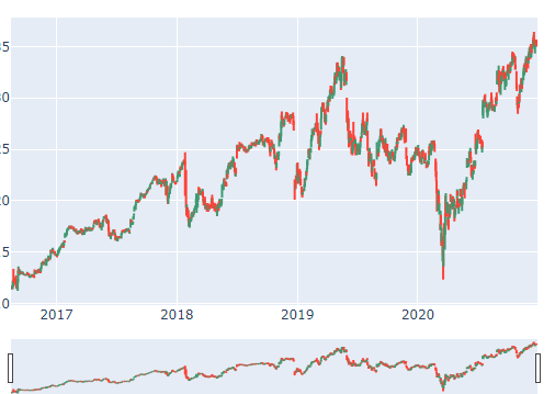
5.2.1 Basic SMA
#DE_Data=DE_Data.reset_index()

DE_Data['SMA5'] = DE_Data.Close.rolling(5).mean()
DE_Data['SMA20'] = DE_Data.Close.rolling(20).mean()
DE_Data['SMA50'] = DE_Data.Close.rolling(50).mean()
DE_Data['SMA200'] = DE_Data.Close.rolling(200).mean()
DE_Data['SMA500'] = DE_Data.Close.rolling(500).mean()

fig = go.Figure(data=[go.Ohlc(x=DE_Data['Date'],open=DE_Data['Open'],high=DE_Data['High'],low=DE_Data['Low'],close=DE_Data['Close'], name = "OHLC"),
                      go.Scatter(x=DE_Data.Date, y=DE_Data.SMA5, line=dict(color='orange', width=1), name="SMA5"),
                      go.Scatter(x=DE_Data.Date, y=DE_Data.SMA20, line=dict(color='green', width=1), name="SMA20"),
                      go.Scatter(x=DE_Data.Date, y=DE_Data.SMA50, line=dict(color='blue', width=1), name="SMA50"),
                      go.Scatter(x=DE_Data.Date, y=DE_Data.SMA200, line=dict(color='violet', width=1), name="SMA200"),
                      go.Scatter(x=DE_Data.Date, y=DE_Data.SMA500, line=dict(color='purple', width=1), name="SMA500")])
fig.show()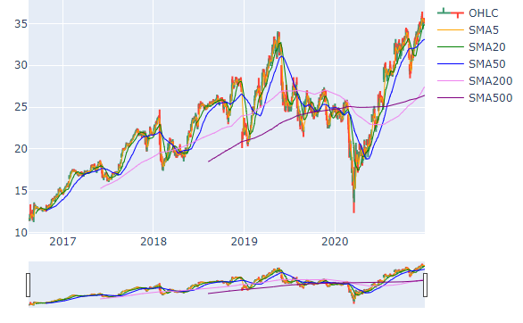
5.2.2 Basic EMA
DE_Data['EMA5'] = DE_Data.Close.ewm(span=5, adjust=False).mean()
DE_Data['EMA20'] = DE_Data.Close.ewm(span=20, adjust=False).mean()
DE_Data['EMA50'] = DE_Data.Close.ewm(span=50, adjust=False).mean()
DE_Data['EMA200'] = DE_Data.Close.ewm(span=200, adjust=False).mean()
DE_Data['EMA500'] = DE_Data.Close.ewm(span=500, adjust=False).mean()

fig = go.Figure(data=[go.Ohlc(x=DE_Data['Date'],
                              open=DE_Data['Open'],
                              high=DE_Data['High'],
                              low=DE_Data['Low'],
                              close=DE_Data['Close'], name = "OHLC"),
                      go.Scatter(x=DE_Data.Date, y=DE_Data.SMA5, line=dict(color='orange', width=1), name="EMA5"),
                      go.Scatter(x=DE_Data.Date, y=DE_Data.SMA20, line=dict(color='green', width=1), name="EMA20"),
                      go.Scatter(x=DE_Data.Date, y=DE_Data.SMA50, line=dict(color='blue', width=1), name="EMA50"),
                      go.Scatter(x=DE_Data.Date, y=DE_Data.SMA200, line=dict(color='violet', width=1), name="EMA200"),
                      go.Scatter(x=DE_Data.Date, y=DE_Data.SMA500, line=dict(color='purple', width=1), name="EMA500")])
fig.show()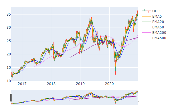
DE_Data.head()
Out[18]:
| Date | Open | High | Low | Close | Volume | Dividends | Stock Splits | 42 | 252 | SMA5 | SMA20 | SMA50 | SMA200 | SMA500 | EMA5 | EMA20 | EMA50 | EMA200 | EMA500 | |
|---|---|---|---|---|---|---|---|---|---|---|---|---|---|---|---|---|---|---|---|---|
| 0 | 2016-08-17 00:00:00-04:00 | 11.636467 | 11.770219 | 11.502714 | 11.502714 | 271519 | 0 | 0.0 | NaN | NaN | NaN | NaN | NaN | NaN | NaN | 11.502714 | 11.502714 | 11.502714 | 11.502714 | 11.502714 |
| 1 | 2016-08-18 00:00:00-04:00 | 11.770218 | 11.770218 | 11.368961 | 11.435837 | 1767366 | 0 | 0.0 | NaN | NaN | NaN | NaN | NaN | NaN | NaN | 11.480422 | 11.496345 | 11.500092 | 11.502049 | 11.502447 |
| 2 | 2016-08-19 00:00:00-04:00 | 11.422462 | 11.636466 | 11.409087 | 11.636466 | 4735900 | 0 | 0.0 | NaN | NaN | NaN | NaN | NaN | NaN | NaN | 11.532436 | 11.509690 | 11.505440 | 11.503386 | 11.502982 |
| 3 | 2016-08-22 00:00:00-04:00 | 11.502714 | 12.198227 | 11.395712 | 11.676593 | 2245909 | 0 | 0.0 | NaN | NaN | NaN | NaN | NaN | NaN | NaN | 11.580489 | 11.525585 | 11.512151 | 11.505110 | 11.503675 |
| 4 | 2016-08-23 00:00:00-04:00 | 11.703343 | 12.278478 | 11.636466 | 12.037724 | 1483020 | 0 | 0.0 | NaN | NaN | 11.657867 | NaN | NaN | NaN | NaN | 11.732901 | 11.574360 | 11.532762 | 11.510409 | 11.505807 |
6 FINTA Tech Analysis Ratios
Let us do a financial ratios calculation using FINTA library
- Simple Moving Average ‘SMA’
- Simple Moving Median ‘SMM’
- Smoothed Simple Moving Average ‘SSMA’
- Exponential Moving Average ‘EMA’
- Double Exponential Moving Average ‘DEMA’
- Triple Exponential Moving Average ‘TEMA’
- Triangular Moving Average ‘TRIMA’
- Triple Exponential Moving Average Oscillator ‘TRIX’
- Volume Adjusted Moving Average ‘VAMA’
- Kaufman Efficiency Indicator ‘ER’
- Kaufman’s Adaptive Moving Average ‘KAMA’
- Zero Lag Exponential Moving Average ‘ZLEMA’
- Weighted Moving Average ‘WMA’
- Hull Moving Average ‘HMA’
- Elastic Volume Moving Average ‘EVWMA’
- Volume Weighted Average Price ‘VWAP’
- Smoothed Moving Average ‘SMMA’
- Fractal Adaptive Moving Average ‘FRAMA’
- Moving Average Convergence Divergence ‘MACD’
- Percentage Price Oscillator ‘PPO’

- Volume-Weighted MACD ‘VW_MACD’
- Elastic-Volume weighted MACD ‘EV_MACD’
- Market Momentum ‘MOM’
- Rate-of-Change ‘ROC’
- Relative Strenght Index ‘RSI’
- Inverse Fisher Transform RSI ‘IFT_RSI’
- True Range ‘TR’
- Average True Range ‘ATR’
- Stop-and-Reverse ‘SAR’
- Bollinger Bands ‘BBANDS’
- Bollinger Bands Width ‘BBWIDTH’
- Momentum Breakout Bands ‘MOBO’
- Percent B ‘PERCENT_B’
- Keltner Channels ‘KC’
- Donchian Channel ‘DO’
- Directional Movement Indicator ‘DMI’
- Average Directional Index ‘ADX’
- Pivot Points ‘PIVOT’
- Fibonacci Pivot Points ‘PIVOT_FIB’
- Stochastic Oscillator %K ‘STOCH’
- Stochastic oscillator %D ‘STOCHD’
- Stochastic RSI ‘STOCHRSI’
- Williams %R ‘WILLIAMS’
- Ultimate Oscillator ‘UO’
- Awesome Oscillator ‘AO’
- Mass Index ‘MI’
- Vortex Indicator ‘VORTEX’
- Know Sure Thing ‘KST’
- True Strength Index ‘TSI’
- Typical Price ‘TP’
- Accumulation-Distribution Line ‘ADL’
- Chaikin Oscillator ‘CHAIKIN’
- Money Flow Index ‘MFI’
- On Balance Volume ‘OBV’
- Weighter OBV ‘WOBV’
- Volume Zone Oscillator ‘VZO’
- Price Zone Oscillator ‘PZO’
- Elder’s Force Index ‘EFI’
- Cummulative Force Index ‘CFI’
- Bull power and Bear Power ‘EBBP’
- Ease of Movement ‘EMV’
- Commodity Channel Index ‘CCI’
- Coppock Curve ‘COPP’
- Buy and Sell Pressure ‘BASP’
- Normalized BASP ‘BASPN’


- Chande Momentum Oscillator ‘CMO’
- Chandelier Exit ‘CHANDELIER’
- Qstick ‘QSTICK’
- Twiggs Money Index ‘TMF’
- Wave Trend Oscillator ‘WTO’
- Fisher Transform ‘FISH’
- Ichimoku Cloud ‘ICHIMOKU’
- Adaptive Price Zone ‘APZ’
- Squeeze Momentum Indicator ‘SQZMI’
- Volume Price Trend ‘VPT’
- Finite Volume Element ‘FVE’
- Volume Flow Indicator ‘VFI’
- Moving Standard deviation ‘MSD’
- Schaff Trend Cycle ‘STC’
try:
    from finta import TA
    from backtesting import Backtest, Strategy
    from backtesting.lib import crossover
except:
    !pip install finta backtesting
    from finta import TA
    from backtesting import Backtest, Strategy
    from backtesting.lib import crossover
try:
from finta import TA
from backtesting import Backtest, Strategy
from backtesting.lib import crossover
except:
!pip install finta backtesting
from finta import TA
from backtesting import Backtest, Strategy
from backtesting.lib import crossover
fin_ma = pd.read_csv('../input/dell-stock-data-latest-and-updated/DELL_stock_history.csv',
parse_dates=True,
sep='\t')
print(fin_ma.head())
ohlc=fin_ma
print(TA.SMA(ohlc, 42))
#ohlc.index = ohlc[index].dt.datefunction_dict = {' Simple Moving Average ' : 'SMA',
' Simple Moving Median ' : 'SMM',
' Smoothed Simple Moving Average ' : 'SSMA',
' Exponential Moving Average ' : 'EMA',
' Double Exponential Moving Average ' : 'DEMA',
' Triple Exponential Moving Average ' : 'TEMA',
' Triangular Moving Average ' : 'TRIMA',
' Triple Exponential Moving Average Oscillator ' : 'TRIX',
' Volume Adjusted Moving Average ' : 'VAMA',
' Kaufman Efficiency Indicator ' : 'ER',
#' Kaufmans Adaptive Moving Average ' : 'KAMA',
#' Zero Lag Exponential Moving Average ' : 'ZLEMA',
' Weighted Moving Average ' : 'WMA',
' Hull Moving Average ' : 'HMA',
#' Elastic Volume Moving Average ' : 'EVWMA',
' Volume Weighted Average Price ' : 'VWAP',
' Smoothed Moving Average ' : 'SMMA',
' Fractal Adaptive Moving Average ' : 'FRAMA',
' Moving Average Convergence Divergence ' : 'MACD',
' Percentage Price Oscillator ' : 'PPO',
' Volume-Weighted MACD ' : 'VW_MACD',
#' Elastic-Volume weighted MACD ' : 'EV_MACD',
' Market Momentum ' : 'MOM',
' Rate-of-Change ' : 'ROC',
' Relative Strength Index ' : 'RSI',
' Inverse Fisher Transform RSI ' : 'IFT_RSI',
' True Range ' : 'TR',
' Average True Range ' : 'ATR',
' Stop-and-Reverse ' : 'SAR',
' Bollinger Bands ' : 'BBANDS',
' Bollinger Bands Width ' : 'BBWIDTH',
' Momentum Breakout Bands ' : 'MOBO',
' Percent B ' : 'PERCENT_B',
' Keltner Channels ' : 'KC',
' Donchian Channel ' : 'DO',
' Directional Movement Indicator ' : 'DMI',
' Average Directional Index ' : 'ADX',
' Pivot Points ' : 'PIVOT',
' Fibonacci Pivot Points ' : 'PIVOT_FIB',
' Stochastic Oscillator Percent K ' : 'STOCH',
' Stochastic oscillator Percent D ' : 'STOCHD',
' Stochastic RSI ' : 'STOCHRSI',
' Williams Percent R ' : 'WILLIAMS',
' Ultimate Oscillator ' : 'UO',
' Awesome Oscillator ' : 'AO',
' Mass Index ' : 'MI',
#' Vortex Indicator ' : 'VORTEX',
' Know Sure Thing ' : 'KST',
' True Strength Index ' : 'TSI',
' Typical Price ' : 'TP',
' Accumulation-Distribution Line ' : 'ADL',
' Chaikin Oscillator ' : 'CHAIKIN',
' Money Flow Index ' : 'MFI',
' On Balance Volume ' : 'OBV',
' Weighter OBV ' : 'WOBV',
' Volume Zone Oscillator ' : 'VZO',
' Price Zone Oscillator ' : 'PZO',
' Elders Force Index ' : 'EFI',
' Cummulative Force Index ' : 'CFI',
' Bull power and Bear Power ' : 'EBBP',
' Ease of Movement ' : 'EMV',
' Commodity Channel Index ' : 'CCI',
' Coppock Curve ' : 'COPP',
' Buy and Sell Pressure ' : 'BASP',
' Normalized BASP ' : 'BASPN',
' Chande Momentum Oscillator ' : 'CMO',
' Chandelier Exit ' : 'CHANDELIER',
' Qstick ' : 'QSTICK',
#' Twiggs Money Index ' : 'TMF',
' Wave Trend Oscillator ' : 'WTO',
' Fisher Transform ' : 'FISH',
' Ichimoku Cloud ' : 'ICHIMOKU',
' Adaptive Price Zone ' : 'APZ',
#' Squeeze Momentum Indicator ' : 'SQZMI',
' Volume Price Trend ' : 'VPT',
' Finite Volume Element ' : 'FVE',
' Volume Flow Indicator ' : 'VFI',
' Moving Standard deviation ' : 'MSD',
' Schaff Trend Cycle ' : 'STC'}
for key, value in function_dict .items():
function_name = "TA." + value + "(ohlc).plot(title='" + key + "for DELL Stock')"
print(function_name)
result = eval(function_name)


7 Back Testing Trading Strategy
# Defining DEMA cross strategy
class DemaCross(Strategy):

    def init(self):

        self.ma1 = self.I(TA.DEMA, ohlc, 10)
        self.ma2 = self.I(TA.DEMA, ohlc, 20)

    def next(self):
        if crossover(self.ma1, self.ma2):
            self.buy()
        elif crossover(self.ma2, self.ma1):
            self.sell()
Let us do a bit of backtesting with a value of $100000
ohlc.head()
print(ohlc.Date)
bt = Backtest(ohlc, DemaCross,
cash=100000, commission=0.015, exclusive_orders=True)!pip uninstall bokeh --yes
!pip install bokeh==3.2.1Back Testing Summary
bt.run()
As you can see, if you had invested $100,000 in DELL shares, you would have got by now a return of 38%! with a peak value of $216,477
data=ohlc
from backtesting import Strategy
from backtesting.lib import crossover
from backtesting.test import SMA
def BBANDS(data, n_lookback, n_std):
    """Bollinger bands indicator"""
    hlc3 = (data.High + data.Low + data.Close) / 3
    mean, std = hlc3.rolling(n_lookback).mean(), hlc3.rolling(n_lookback).std()
    upper = mean + n_std*std
    lower = mean - n_std*std
    return upper, lower


close = data.Close.values
sma10 = SMA(data.Close, 10)
sma20 = SMA(data.Close, 20)
sma50 = SMA(data.Close, 50)
sma100 = SMA(data.Close, 100)
upper, lower = BBANDS(data, 20, 2)

# Design matrix / independent features:

# Price-derived features
data['X_SMA10'] = (close - sma10) / close
data['X_SMA20'] = (close - sma20) / close
data['X_SMA50'] = (close - sma50) / close
data['X_SMA100'] = (close - sma100) / close

data['X_DELTA_SMA10'] = (sma10 - sma20) / close
data['X_DELTA_SMA20'] = (sma20 - sma50) / close
data['X_DELTA_SMA50'] = (sma50 - sma100) / close

# Indicator features
data['X_MOM'] = data.Close.pct_change(periods=2)
data['X_BB_upper'] = (upper - close) / close
data['X_BB_lower'] = (lower - close) / close
data['X_BB_width'] = (upper - lower) / close
#data['X_Sentiment'] = ~data.index.to_series().between('2017-09-27', '2017-12-14')

# Some datetime features for good measure
#data['X_day'] = data.index.dayofweek
#data['X_hour'] = data.index.hour

#data = data.apply(pd.to_numeric)
#data = data.dropna().astype(np.float64)
#data.fillna(method="ffill")
#data =data[~data.isin([np.nan, np.inf, -np.inf]).any(1)]

#data.replace([np.inf, -np.inf], 0.0, inplace=True)
#data = data.fillna(data.mean(), inplace=True)
#data = data.dropna().astype(np.float64)
class Sma4Cross(Strategy):
n1 = 50
n2 = 100
n_enter = 20
n_exit = 10
def init(self):
self.sma1 = self.I(SMA, self.data.Close, self.n1)
self.sma2 = self.I(SMA, self.data.Close, self.n2)
self.sma_enter = self.I(SMA, self.data.Close, self.n_enter)
self.sma_exit = self.I(SMA, self.data.Close, self.n_exit)
def next(self):
if not self.position:
# On upwards trend, if price closes above
# "entry" MA, go long
# Here, even though the operands are arrays, this
# works by implicitly comparing the two last values
if self.sma1 > self.sma2:
if crossover(self.data.Close, self.sma_enter):
self.buy()
# On downwards trend, if price closes below
# "entry" MA, go short
else:
if crossover(self.sma_enter, self.data.Close):
self.sell()
# But if we already hold a position and the price
# closes back below (above) "exit" MA, close the position
else:
if (self.position.is_long and
crossover(self.sma_exit, self.data.Close)
or
self.position.is_short and
crossover(self.data.Close, self.sma_exit)):
self.position.close()
%%time

from backtesting import Backtest
from backtesting.test import GOOG


backtest = Backtest(ohlc, Sma4Cross, commission=.002)

stats, heatmap = backtest.optimize(
    n1=range(10, 110, 10),
    n2=range(20, 210, 20),
    n_enter=range(15, 35, 5),
    n_exit=range(10, 25, 5),
    constraint=lambda p: p.n_exit < p.n_enter < p.n1 < p.n2,
    maximize='Equity Final [$]',
    max_tries=200,
    random_state=0,
    return_heatmap=True)
CPU times: user 170 ms, sys: 52.4 ms, total: 223 ms Wall time: 3.94 s
heatmap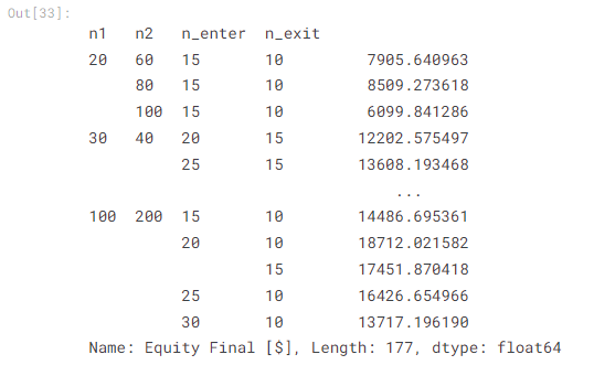
hm = heatmap.groupby(['n1', 'n2']).mean().unstack()
hm| n2 | 40 | 60 | 80 | 100 | 120 | 140 | 160 | 180 | 200 |
|---|---|---|---|---|---|---|---|---|---|
| n1 | |||||||||
| 20 | NaN | 7905.640963 | 8509.273618 | 6099.841286 | NaN | NaN | NaN | NaN | NaN |
| 30 | 12905.384483 | 8200.119386 | 9476.787154 | 10009.929662 | 10184.621792 | 10138.254127 | 8734.760719 | 12446.921112 | 13240.048632 |
| 40 | NaN | 10726.067433 | NaN | 9785.522760 | 8992.199807 | 10550.786743 | 8393.881424 | 11124.085959 | 13053.633516 |
| 50 | NaN | 11485.340283 | 10851.161023 | 8703.910432 | 9231.192470 | 10228.470540 | 11296.825742 | 12663.553557 | 13233.358413 |
| 60 | NaN | NaN | 11374.121060 | 8784.022732 | 9760.689339 | 8140.882026 | 12346.172616 | 12584.163286 | 10558.088613 |
| 70 | NaN | NaN | 10590.552738 | 9798.934944 | 8317.988207 | 11027.718788 | 9579.299147 | 10113.382211 | 12735.625402 |
| 80 | NaN | NaN | NaN | 8688.350774 | 10483.468572 | 7327.781173 | 12166.192714 | 11123.923457 | 12871.204344 |
| 90 | NaN | NaN | NaN | 9471.473045 | 8776.650746 | 7545.290015 | 10677.806685 | 11347.162070 | 11795.845754 |
| 100 | NaN | NaN | NaN | NaN | 6882.797977 | 7185.029985 | 11264.643996 | 12415.991007 | 16158.887703 |
WORK IN PROGRESS
from backtesting.lib import plot_heatmaps

#plot_heatmaps(heatmap, agg='mean')
Conclusion
In the intriguing world of finance, our exploration of DELL stock has unveiled a compelling investment opportunity. Dell Technologies’ enduring presence in the tech sector, along with its diverse product range and consistent financial performance, piques the interest of both seasoned investors and newcomers.
Nonetheless, it’s important to bear in mind that the stock market is an ever-changing landscape, full of surprises.
As you navigate your financial journey, consider diversifying your portfolio and consulting with financial experts to make informed decisions.

In the realm of stocks, one certainty prevails – the future is always full of twists and turns. So, let’s continue watching, learning, and adapting to these dynamic financial markets. Here’s to your investments flourishing and delivering the results you aspire to achieve.
Learn more


0 Comments