Machine Learning Exercise 1: Best Implement Linear Regression from scratch

Sharing is caring!

Introduction

Hey there! 👋 Today, we’re gonna dive into the world of linear regression. Our mission? Predict laptop prices using some cool Python and NumPy magic.

We’ll be working with a dataset of laptops and trying to figure out how their screen size, RAM, and weight affect their price. Ready? Let’s roll! 🚀

The goal of this exercise is to implement a simple Linear Regression model to predict laptop prices based on some numerical features from the dataset. Specifically, we will use the screen size, RAM size, and weight as features.

Let’s Code

Grab the Data 📂

First things first, let’s get that data! Download the dataset from Kaggle and load it up using Pandas.

import pandas as pd

# Load the dataset
data = pd.read_csv('laptop_price.csv')

Clean Up Time (Pre-processing)🧹

Now, we gotta clean the data a bit. We’re gonna turn the Ram and Weight columns into numbers. Let’s get rid of those pesky ‘GB’ and ‘kg’ strings.

# Clean up Ram and Weight columns
data['Ram'] = data['Ram'].str.replace('GB', '').astype(float)
data['Weight'] = data['Weight'].str.replace('kg', '').astype(float)

Pick Your Features (Features Engineering) 🌟

We need to decide what info we’re gonna use to predict prices. Let’s go with Inches, Ram, and Weight. And our target is Price_euros.

# Pick the features and target variable
X = data[['Inches', 'Ram', 'Weight']]
y = data['Price_euros']

Let’s also normalize these features to make our model perform better.

# Normalize the features
X = (X - X.mean()) / X.std()

# Add a column of ones for the bias term
X = np.c_[np.ones(X.shape[0]), X]

# Convert to numpy arrays
X = np.array(X)
y = np.array(y)

Time to Code Linear Regression 🖥️

Alright, let’s break it down. We’ll write some functions to make our linear regression work.

import numpy as np

# Initialize weights
def initialize_weights(n):
    return np.zeros(n)

# Predict output
def predict(X, weights):
    return np.dot(X, weights)

# Compute loss (Mean Squared Error)
def compute_loss(y, y_pred):
    return np.mean((y - y_pred) ** 2)

# Perform gradient descent
def gradient_descent(X, y, weights, learning_rate, epochs):
    m = len(y)
    for _ in range(epochs):
        y_pred = predict(X, weights)
        gradients = -2/m * np.dot(X.T, (y - y_pred))
        weights -= learning_rate * gradients
    return weights

# Initialize weights
weights = initialize_weights(X.shape[1])

# Set hyperparameters
learning_rate = 0.01
epochs = 1000

# Train the model
weights = gradient_descent(X, y, weights, learning_rate, epochs)

Check Out the Results 📈

Let’s see how our model did. We’ll predict the prices and check out the Mean Squared Error (MSE).

# Predict using the trained model
y_pred = predict(X, weights)

# Compute the loss
loss = compute_loss(y, y_pred)
print(f'Mean Squared Error: {loss}')

What is Linear Regression? 🤔

Hey there! 👋 Let’s break down what linear regression is in a super simple way. Imagine you’re a detective 🕵️‍♂️, and your job is to find out how one thing affects another.

For example, you might want to know how the size of a laptop’s screen 📺, the amount of RAM 🧠, and its weight 🏋️‍♂️ impact its price 💰. That’s where linear regression comes in. It’s like your detective toolkit for finding these connections!

Other Example:

Let’s say you have data on laptops, and you want to predict their price based on screen size, RAM, and weight. You’d plot this data, find the best-fitting line, and use that line to predict prices of new laptops.

And that’s the gist of it! Linear regression is like drawing a line through data to predict outcomes. It’s super handy and a great tool to have in your machine learning toolbox. Keep exploring and have fun with it! 🚀

The Basics

Linear regression is a method for predicting a value based on other values. It’s like drawing a straight line through a bunch of points and using that line to guess where new points might be.

How Linear Regression Works

• Features: These are the things you think might affect what you’re trying to predict. In our case, features could be the screen size, RAM, and weight of laptops.
• Target: This is what you’re trying to predict. Here, it’s the price of the laptop.

The Straight Line

In linear regression, we find the best-fitting line through our data points. The line can be represented with this simple equation:

[ y = mx + b ]

• ( y ): This is the target variable (like the laptop price).
• ( x ): These are the features (like screen size, RAM, weight).
• ( m ): This is the slope of the line. It tells us how much ( y ) changes for a one-unit change in ( x ).
• ( b ): This is the y-intercept. It’s where the line crosses the y-axis.

Why Use Linear Regression?

• Simple and Intuitive: It’s easy to understand and implement.
• Quick Insights: You can quickly see how different features impact the target variable.
• Foundation for More Complex Models: It’s a great starting point before diving into more complex machine learning models.

How to Do Linear Regression?

1. Collect Data: Get your data ready. You need a bunch of examples with features and their corresponding target values.
2. Choose Features and Target: Decide which columns are your features and which one is your target.
3. Train Your Model: Use the data to find the best values for ( m ) and ( b ). This is usually done using a method called gradient descent.
4. Make Predictions: Use the model to predict the target for new data points.
5. Evaluate the Model: Check how good your predictions are using metrics like Mean Squared Error (MSE).

Linear regression is a statistical method that models the relationship between two variables by fitting a straight line to the data points. The straight line is called the regression line, and it is used to predict the value of the dependent variable (y) based on the value of the independent variable (x).

The equation for the regression line is:

y = mx + b

where:

• y is the dependent variable
• x is the independent variable
• m is the slope of the line
• b is the y-intercept of the line

The slope (m) tells you how much the y-value changes for every one-unit increase in the x-value. The y-intercept (b) is the point where the regression line crosses the y-axis.

What is an Example of a Linear Regression?

Sure thing! Linear regression is like drawing the best straight line through a bunch of data points. Imagine you wanna predict how much pizza you can eat based on the number of hours you play video games.

Here’s a simple example with some Python code to make it all clear:

# First, import the stuff we need
import numpy as np
import matplotlib.pyplot as plt
from sklearn.linear_model import LinearRegression

# Let's say these are the hours you play video games and the slices of pizza you eat
video_game_hours = np.array([1, 2, 3, 4, 5, 6]).reshape(-1, 1)
pizza_slices = np.array([2, 3, 4, 5, 6, 7])

# Set up the linear regression model
model = LinearRegression()

# Train the model with our data
model.fit(video_game_hours, pizza_slices)

# Now, let's predict pizza slices for those video game hours
predicted_pizza_slices = model.predict(video_game_hours)

# Plotting the results to see the line
plt.scatter(video_game_hours, pizza_slices, color='blue') # the dots (actual data)
plt.plot(video_game_hours, predicted_pizza_slices, color='red') # the line (predicted data)
plt.xlabel('Video Game Hours')
plt.ylabel('Pizza Slices')
plt.title('Video Game Hours vs Pizza Slices')
plt.show()

Here’s what’s happening:

• Step One: Import the needed libraries. Numpy for handling numbers, matplotlib for plotting, and sklearn for the linear regression stuff.
• Step Two: Create arrays for video_game_hours and pizza_slices. These represent the data points. Each pair shows how many hours of gaming equals how many slices of pizza.
• Step Three: Set up the linear regression model with LinearRegression(). This tells Python that we want to use linear regression.
• Step Four: Train the model using model.fit(). We’re feeding it our data so it can learn the relationship between gaming hours and pizza slices.
• Step Five: Use model.predict() to get the predicted pizza slices based on gaming hours. It’s like asking, “If I play this many hours, how many slices should I expect to eat?”
• Step Six: Plot the results. Blue dots are the actual data points, and the red line shows the predicted relationship.

And there you have it! A simple way to see how one thing affects another with linear regression. Now, go ahead and try it with your own data!

When should linear regression be used?

Linear regression is a go-to tool when you need to predict a continuous outcome or understand relationships between variables. Here’s when it’s your best bet:

• Predicting Values: If you want to forecast something like house prices based on square footage, linear regression fits the bill.
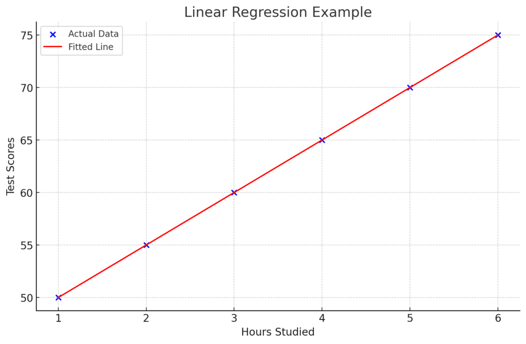
• Simple Relationships: When you think there’s a straight-line relationship between variables, like hours studied and test scores, this method shines.
• Continuous Data: It works best with numerical data that doesn’t fit into categories, such as temperature, age, or income.

In a nutshell, use linear regression when you need a straightforward, interpretable model to predict or explain continuous data based on other continuous inputs. It’s like drawing the best straight line through your data points to make sense of the relationships!

Why use linear regression to predict?

Linear regression is a popular choice for prediction because of its simplicity, interpretability, computational efficiency, and flexibility. It is easy to grasp and apply, making it suitable for a diverse group of users.

Moreover, the coefficients it produces provide valuable insights into how predictors influence the outcome.

This approach remains efficient even when dealing with extensive datasets, making it highly applicable in real-world scenarios.

Although it assumes a linear relationship between variables, it is resilient and does not demand strict assumptions about data distribution. Furthermore, it serves as a reliable benchmark for comparing more intricate models.

How to interpret a linear regression?

In your journey through linear regression, start by exploring the equation itself. It serves as your recipe for making predictions, revealing how the outcome (Y) is influenced by the predictors (Xs). Think of it as ( Y = \beta_0 + \beta_1X + \epsilon ).

Once you understand the equation, delve into its components: the coefficients. The intercept, ( \beta_0 ), sets the starting point, while the slope, ( \beta_1 ), indicates how much Y changes when X moves by one unit.

Next, evaluate their significance by checking if they have statistical importance. If they do, they likely have a meaningful impact on the outcome.

Now, assess how well your model fits the data using ( R^2 ), a measure of “goodness of fit”. Higher ( R^2 ) values suggest a better fit.

Make sure your model meets basic assumptions such as linearity, independence of errors, consistent variance, and normal residuals to ensure its reliability.

If you have included any special features like interaction terms or higher-order terms, examine them closely. They capture more complex relationships between variables.

Lastly, don’t solely focus on statistical significance. Consider practical significance as well. Sometimes, even small changes can have a significant real-world effect.

This approach will help unravel the mysteries of linear regression and shed light on how your variables interact with each other.

What is a good p value in regression?

In regression analysis, the p-value associated with each coefficient helps determine the statistical significance of that predictor variable. A common threshold for considering a p-value as “good” or statistically significant is 0.05.

Here’s what it means:

• p-value < 0.05: If the p-value is less than 0.05, it suggests that the coefficient is statistically significant. In other words, there is strong evidence to reject the null hypothesis, indicating that the predictor variable has a significant effect on the outcome variable.
• p-value ≥ 0.05: If the p-value is greater than or equal to 0.05, it implies that the coefficient is not statistically significant. In this case, there isn’t enough evidence to reject the null hypothesis, suggesting that the predictor variable may not have a significant effect on the outcome variable.

However, it’s essential to consider the context of your analysis and the specific field you’re working in. In some cases, a more conservative threshold (e.g., p < 0.01) might be appropriate, especially in fields where false positives are particularly problematic. Conversely, in exploratory analyses or fields where hypotheses are often tested, a slightly higher threshold might be acceptable.

Ultimately, the choice of the “good” p-value depends on the research question, the study design, and the prevailing standards in the field.

Can the p value be negative?

No, p-values cannot be negative.

A p-value is a probability that represents the likelihood of observing the data (or more extreme data) given that the null hypothesis is true. It is always a value between 0 and 1.

A p-value less than 0.05 suggests that the observed data are unlikely to have occurred under the assumption of the null hypothesis, leading to its rejection in favor of the alternative hypothesis.

Conversely, a p-value greater than 0.05 indicates that the observed data are reasonably likely to occur under the null hypothesis, and thus, there is insufficient evidence to reject it.

Negative p-values would not make sense in this context and are not used in statistical inference.

How to interpret r squared?

The coefficient of determination, often denoted as ( R^2 ), is a statistical measure that represents the proportion of the variance in the dependent variable (outcome) that is explained by the independent variables (predictors) in a regression model. Here’s how to interpret ( R^2 ):

• ( R^2 ) Value: ( R^2 ) ranges from 0 to 1, where:
• ( R^2 = 0 ): None of the variability in the dependent variable is explained by the independent variables. The model doesn’t fit the data at all.
• ( R^2 = 1 ): All of the variability in the dependent variable is explained by the independent variables. The model perfectly fits the data.
• Interpretation:
• The higher the ( R^2 ) value, the better the model fits the data. For example, an ( R^2 ) of 0.80 indicates that 80% of the variability in the dependent variable is explained by the independent variables in the model.
• Conversely, a lower ( R^2 ) value suggests that the model does not explain much of the variability in the dependent variable.
• Context Matters: While a high ( R^2 ) is desirable, it’s essential to interpret it in the context of your specific research question and the field you’re working in. Some phenomena may inherently have more variability than others, making it harder to achieve a high ( R^2 ). Additionally, ( R^2 ) should be interpreted alongside other metrics and considerations, such as the practical significance of the predictors and the appropriateness of the model assumptions.

Overall, ( R^2 ) provides a useful measure of how well the regression model explains the variability in the data, but it should be interpreted thoughtfully and in conjunction with other information.

Can R^2 be negative?

No, ( R^2 ) cannot be negative.

The coefficient of determination, ( R^2 ), is a measure of how well the independent variables explain the variability of the dependent variable in a regression model. It ranges from 0 to 1, where:

• ( R^2 = 0 ) indicates that the model does not explain any of the variability in the dependent variable.
• ( R^2 = 1 ) indicates that the model perfectly explains all the variability in the dependent variable.

A negative value for ( R^2 ) would not make sense in the context of regression analysis because it would imply that the model performs worse than simply using the mean of the dependent variable to predict outcomes. However, in practice, it’s not possible to obtain a negative ( R^2 ) value when using standard regression techniques.

Conclusion

Feeling adventurous? 🎉 Try these extra challenges!

• Train-Test Split: Split your data into training and testing sets. See how your model does on data it hasn’t seen before.
• Hyperparameter Tuning: Play around with different learning rates and number of epochs. See what works best!
• Feature Engineering: Add more features and see if your predictions get better.

And there you have it! You just built a linear regression model from scratch. High five! ✋ Keep experimenting and have fun with it. 🚀